Forecast demand and size a safety buffer without hiding uncertainty
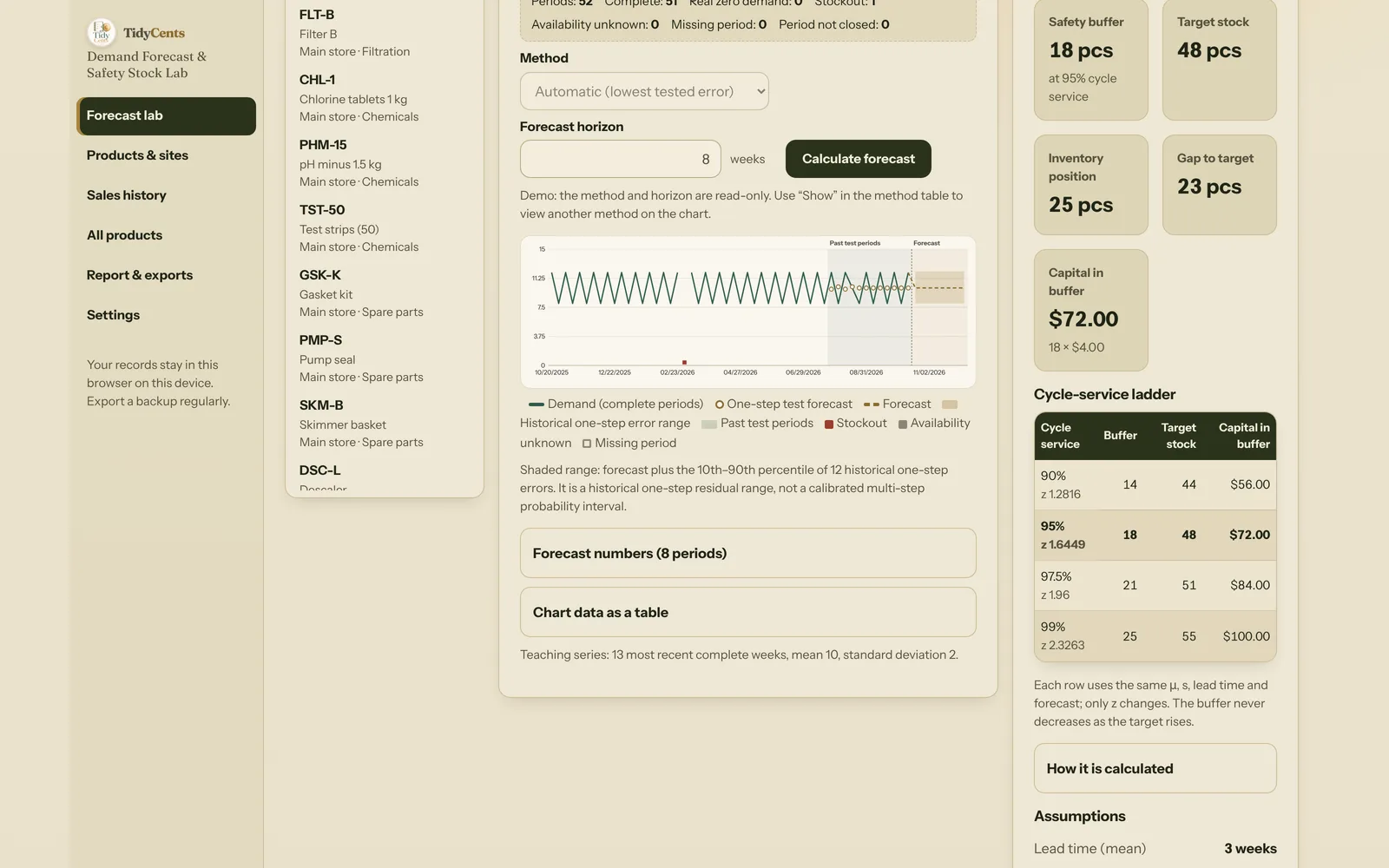
A stock plan begins with two different questions: what demand might occur, and what buffer you are willing to finance if reality differs. Combining them into one unexplained reorder number hides the assumptions that matter. In the worked example below, a product that sells about 10 units a week ends up with a safety buffer of 18 units, a target stock of 48, a gap of 23 units to that target — and $72 of cash tied up in the buffer alone. Every one of those numbers comes from an assumption you can see and change.
Start with usable history
A genuine zero-sales week is information. A week when the product was unavailable is not evidence that nobody wanted it. If a filter sold out on Tuesday and nothing was sold for the rest of the week, recording that week as "0" teaches every forecasting method that demand fell — and the next buffer will be too small exactly where you already ran out.
So mark those periods separately:
- Complete period — the product was available and the period is closed. A zero here is a real zero.
- Stockout — the product ran out. The period is a gap, not a zero.
- Unknown availability — you cannot tell. Also a gap.
- Open period — the current week that is still running. It is forecast, not used as history.
Missing dates should not silently become zeros either. If your export skipped two weeks because a store's till was offline, those weeks are missing, not "no sales". And returns are not negative demand: correct the source history first (for example, net returns out of the week of the original sale) and write down how you did it.
In the fictional demo shop, one product had two stockout weeks and one week of unknown availability in the last few months. Its most recent unbroken run of complete weeks is only 11 long — so the tool refuses to estimate a buffer from it rather than pretending the gaps were zeros.
Compare simple methods before adding complexity
A last-value forecast, a moving average, exponential smoothing and a seasonal repeat can produce very different results from the same history. The honest way to choose is to test eligible methods on the same past periods, training each prediction only on information available before its date. Otherwise the evaluation leaks the answer into the forecast.
A rolling-origin test does exactly this. Take the last 12 complete weeks (or a quarter of the history, whichever is smaller — and at least 4). For each of those weeks, fit every method on the weeks before it and forecast one step ahead. Then compare the misses.
For the demo's teaching product, "Filter A", with 52 weeks of history (one of them a stockout), the one-step test over the same 12 past weeks gave:
| Method | Mean absolute error |
|---|---|
| Moving average, 13 weeks | 1.885 |
| Exponential smoothing, α 0.1 | 1.939 |
| Croston-SBA, α 0.1 | 1.971 |
| Moving average, 8 weeks | 2.000 |
| Moving average, 4 weeks | 2.000 |
| Last value | 3.667 |
The 13-week moving average wins, and its forecast is a flat 10 units a week. Note what is not in the table: the 52-week seasonal repeat. It needs two full years of complete history — 104 weeks — and this product has 51 complete weeks. A tool that still showed a "seasonal forecast" here would be inventing a pattern it has never seen twice.
Two rules keep such a comparison fair. First, a method is ranked only if it could be used at every test period; if a moving average cannot be computed in a week whose window contains a stockout, it does not get a score on fewer, easier weeks. Second, ties are broken by a fixed rule (lower RMSE, then a fixed order), so re-importing the same file in a different row order gives the same answer.
Use an error you can interpret
Mean absolute error describes the average size of a miss in demand units: "we are typically 1.9 units off". Bias shows the direction of the misses — a forecast that is consistently too high fills the shelf with cash. RMSE punishes large misses more than small ones.
Percentage errors require care when actual demand is zero. Weighted absolute percentage error (total absolute error divided by total actual demand) is useful for comparing products of different sizes, but when actual demand in the test weeks is zero the denominator is missing. A model should not display a reassuring zero percentage because its denominator is missing; the honest answer is "unavailable".
Also be clear about what the test measures: it is a one-step-ahead test. It tells you how well a method predicted next week from the weeks before. It does not certify the accuracy of a forecast six months out.
Keep the forecast range honest
A shaded band around a forecast looks reassuring. For Filter A, the 10th and 90th percentiles of the 12 historical one-step errors were −2 and +2.14, which puts next week's range at about 8 to 12.1 units. That is useful context, but label it for what it is: a historical one-step residual range, not a calibrated probability interval for a six-month prediction. With fewer than 8 test errors there are simply too few to calculate it, and no band should be drawn.
Then examine the buffer
The buffer is a separate, approximate model. It makes assumptions you should confirm explicitly: demand and delivery time are independent and non-negative, their parameters are stable enough, and a normal approximation is acceptable. Under those assumptions, variation in both demand and delivery time contributes to uncertainty over the protection period — the lead time plus the review interval.
Suppose mean demand is ten units per period, demand standard deviation is two, mean lead time is three periods and lead-time standard deviation is one, with continuous review. Then:
- Protection periods: T = 3 + 0 = 3
- Variance: V = T·s² + μ²·sL² = 3 × 2² + 10² × 1² = 12 + 100 = 112
- Standard deviation: σ = √112 ≈ 10.583
- At a 95% cycle-service setting, z = 1.644853627, so z·σ ≈ 17.41, rounded up to a whole-unit safety buffer of 18
With a flat forecast of 10 units, expected protection demand over the 3 periods is 30, and the target stock is 30 + 17.41, rounded up to 48.
Notice where the variance comes from: 12 of the 112 come from week-to-week demand, 100 from the uncertain lead time. Shortening or stabilising delivery often does more for the buffer than any forecasting method.
Two practical details matter. If the lead time is entered in days but history is weekly, convert days to weeks first (18 days is 2.57 weeks) and only then round the protection period up; a 2.57-week lead time with a one-week review becomes 4 protection weeks, and the result should say it was rounded. And for products sold by weight or volume, round the buffer up to the step you actually stock, such as half a litre.
Price the buffer and find the gap
If inventory position — on hand plus on order minus backorders — is 20 + 10 − 5 = 25, the gap to that target is 23 units. At $4 per unit, the buffer alone ties up $72.
A ladder of service targets makes the trade-off concrete for the same product:
| Cycle service | Buffer | Target stock | Capital in buffer |
|---|---|---|---|
| 90% | 14 | 44 | $56 |
| 95% | 18 | 48 | $72 |
| 97.5% | 21 | 51 | $84 |
| 99% | 25 | 55 | $100 |
Moving from 95% to 99% costs another $28 of stock for this one product. Across a catalogue of a few hundred products and several locations, that is the conversation worth having with numbers in front of you.
This is an assumption-based planning result, not a purchase order or a guarantee of customer fill rate. "95% cycle service" means roughly 95% of replenishment cycles are expected to end without running out under the stated assumptions — not that 95% of units will be delivered.
Putting it together
Demand Forecast & Safety Stock Lab keeps the forecast, the historical test and the buffer economics connected. Its fixed demo shows a small catalogue and a medium-sized multi-location example with 240 products across 4 locations and 104 weeks, where each product gets its own tested method and buffer capital is totalled per currency. Use Stock Purchase Planner for the subsequent question of packs, minimum quantities and a constrained purchase budget.
Tools mentioned in this guide
 Interactive tool
Demand Forecast & Safety Stock Lab
Forecast demand with transparent statistical methods, check past prediction errors and compare the cash cost of a safety buffer.